Compare the performance of a Metropolis

a. Generate Metropolis-Hastings samples from this density using a range of independent beta candidates from a Be(1, 1) to a beta distribution with small variance. Compare the acceptance rates of the algorithms.

b. Suppose that we want to generate a truncated beta Be(2.7, 6.3) restricted to the interval (c, d) with c, d ∈ (0, 1). Compare the performance of a Metropolis- Hastings algorithm based on a Be(2, 6) proposal with one based on a U(c, d) proposal. Take c = .1, .25 and d = .9, .75.

Example 2.7

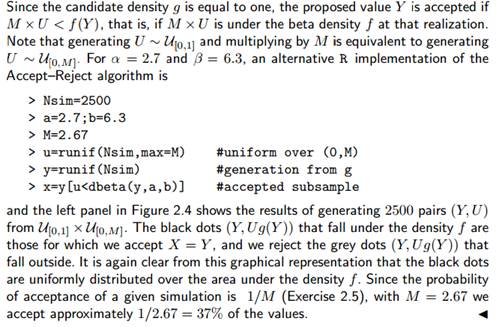
Example 2.2 did not provide a general algorithm to simulate beta Be(α, β) random variables. We can, however, construct a toy algorithm based on the Accept-Reject method, using as the instrumental distribution the uniform U[0,1] distribution when both α and β are larger than 1. (The generic rbeta function does not impose this restriction.) The upper bound M is then the maximum of the beta density, obtained for instance by optimize (or its alias optimise):

> optimize(f=function(x){dbeta(x,2.7,6.3)},
+ interval=c(0,1),max=T)$objective
[1] 2.669744